Killing the Frankenstein Estimate: Bayesian vs. Frequentist Retirement Planning

Why feeding static historical averages into retirement models sets clients up for failure, and how tracking parameter uncertainty changes the game.

1 Introduction

You don’t need to look further than the nearest investment forum to see that discussions inevitably default to expected returns. Soon after, risk enters the chat in the form of volatility, and we find ourselves debating Sharpe, Sortino, or Information ratios.

Institutional investors are particularly sensitive to risk management—and to the specific metrics they market. This is why we get massive annual outlooks detailing expected market returns and projected volatilities. A vast body of financial literature relies heavily on this historical data to inform future backtests. To deal with the inherent uncertainty of the future, analysts frequently use Monte Carlo simulations. Yet, even in their simplest forms, these simulations require rigid point estimates for average return and volatility.

Therein lies a major limitation. We cannot guarantee that historical averages or volatilities are stationary, nor do standard simulations allow us to inform the model with our prior beliefs. Because of this, financial planners who genuinely care about their clients often resort to “Frankenstein” point estimates—fusing historical data and current market indicators together to craft a single, reasonable-looking baseline.

Wouldn’t it be better to use entire distributions that reflect how certain we are about those parameters, rather than running simulations based on fixed numbers?

What I am suggesting is that we stop feeding our models static historical figures or arbitrary mixtures of data. Instead, we should feed them parameter distributions that can evolve as real data arrives. This unlocks a powerful way to look at risk. In a later post, I will explore how this allows for a clean split between epistemological and aleatory risk attribution—essentially quantifying whether a retirement plan failed due to wrongly chosen model parameters or simply a run of terrible luck.

For the upcoming example, I took MSCI World returns in USD from 2012 to 2026 and ran side-by-side frequentist and Bayesian simulations, assuming zero transaction costs.

2 Motivation

In this post, I want to pit the omnipresent frequentist framework against a Bayesian alternative over a 30-year retirement simulation. We will look at how each framework impacts success rates and safe vs. sustainable withdrawal rates at different percentages.

For the setup, I will assume a starting portfolio of $1,000,000 (in real dollars) and an initial withdrawal rate of 2.7%, a slight nod to Ben Felix’s recent work on safe withdrawal rates. Both models will have access to the 2012–2026 MSCI World data, and both will assume a stationary annual inflation rate of 2.5%.

The models differ entirely in how they view parameters:

• The Frequentist Framework: Derives static, historical point estimates for annual real market returns and volatility directly from the dataset.
• The Bayesian Framework: Integrates the data alongside the following explicit prior beliefs:
  • An expected 4.2% real stock market return, with an uncertainty of roughly \(\pm\) 4% modeled as a normal distribution.
  • An expected 16% volatility, with its uncertainty modeled via a Half-Student-\(t\) distribution.

3 Results

Now we get to the interesting part. I simulated classic frequentist Monte Carlo paths alongside Bayesian retirement paths¹ built on our priors and the 2012–2026 MSCI World data.

¹ For all intents and purposes, these can be interpreted as standard retirement trajectories.

² The rate where 95% of portfolios finish the simulated period with a non-negative balance.

³ The rate at which the initial principal capital is fully preserved in 95% of portfolios at the end of the simulation.

In the visualization below, I intentionally plotted a few failed paths to ensure the visual dispersion remains coherent with the calculated success rates. I also calculated the medoid path, the safe withdrawal rate (SWR)², and the sustainable withdrawal rate (SuWR)³. The actual historical baseline and the real withdrawal amounts are traced for context.

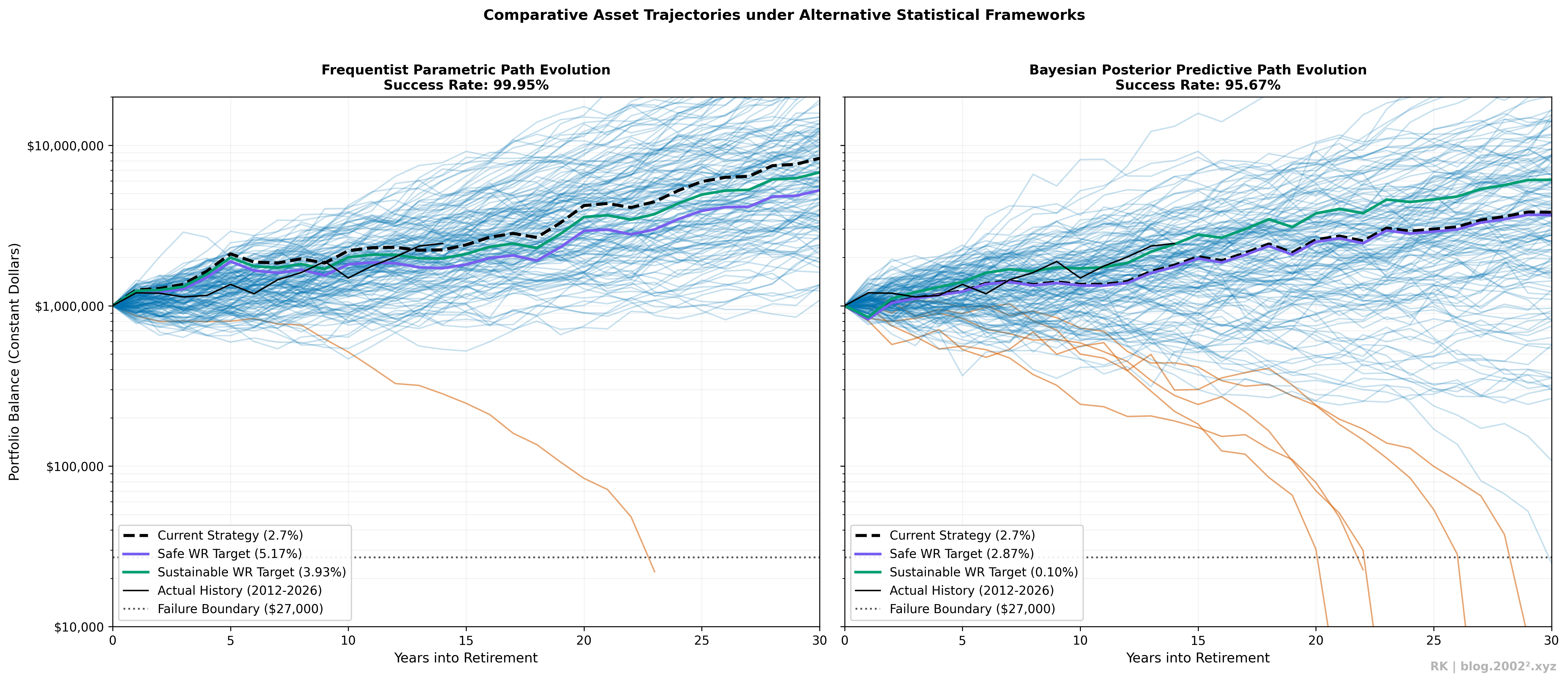
What does this tell us? First, it illustrates why investing over longer time horizons is inherently riskier: the potential outcomes fan out dramatically over time. Second, it highlights the severe recency bias embedded in the frequentist model. Because the 2012–2026 period was exceptionally strong for global equities, the frequentist model yields a staggering 99.95% success rate at a 2.7% withdrawal rate. Under this framework, the Safe Withdrawal Rate climbs to 5.17%, and the Sustainable Withdrawal Rate sits near 4%.

I would argue that the Bayesian framework provides a far more realistic long-term perspective. At a 2.7% withdrawal rate, we are acting safely relative to the model’s calculated 2.87% SWR. However, the sustainable withdrawal rate completely falls off a cliff, dropping to 0.1%. When financial data is noisy or spans a relatively short historical window, Bayesian frameworks yield results that remain structurally anchored by our broader prior beliefs rather than over-fitting to recent market euphoria.

This is a highly desirable characteristic for financial planning tools.

For those interested in the underlying distribution, I have mapped out the dispersion cones below. A quick word of warning: do not confuse confidence cones with credibility cones.

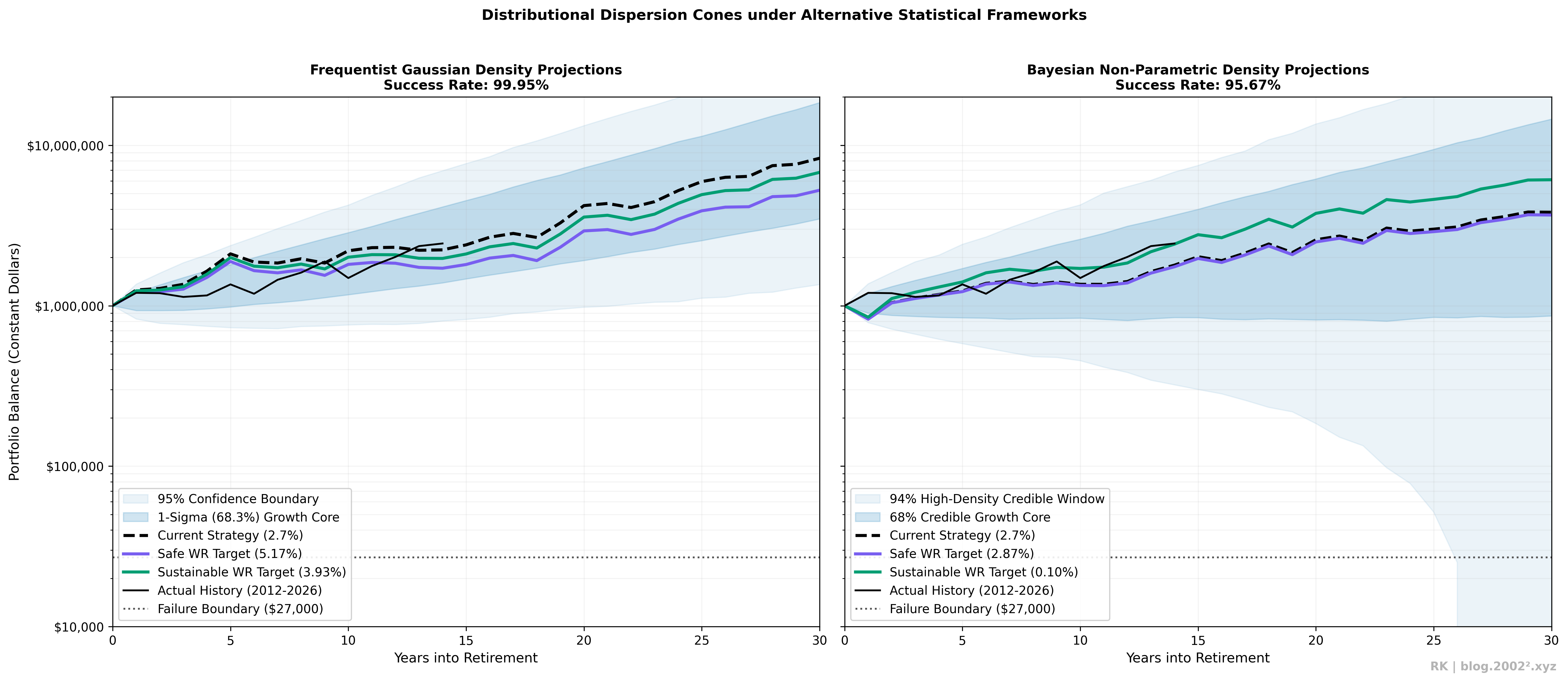
One might fairly counter that these methods aren’t all that different; if you simply fed more conservative historical parameters into the frequentist model, you could match the Bayesian output. That is a reasonable point. But the true advantage of the Bayesian approach is what it exposes under the hood. Let me show you a small amuse-bouche:

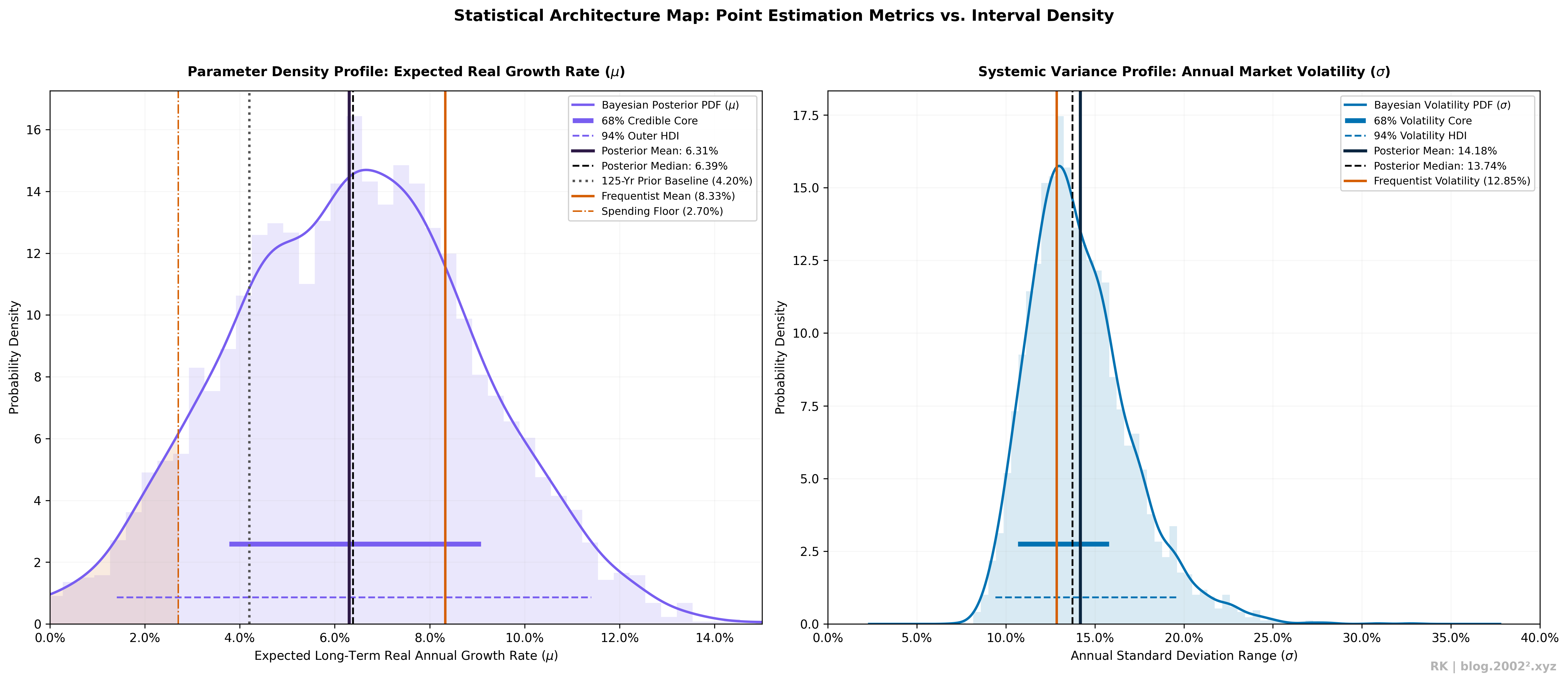
Frequentist models give us isolated point estimates. What we actually want to understand is the uncertainty surrounding those parameters, as well as the joint distribution of returns and volatility.

In this example, we can see exactly why certain withdrawal rates failed in the Bayesian model: the simulated average return (\(\mu\)) was structurally inferior to the required retirement spending drag. With this layer of information, we can go one step further. We can analyze the failed paths and cleanly attribute the failures to either aleatory risk⁴ or epistemological risk⁵.

⁴ Think of this as pure sequence-of-returns risk.

⁵ Think of this as a structurally unlucky draw where the underlying economy performed worse than expected.

4 Conclusion

The frequentist approach is simply the wrong tool in our statistical toolbox for pragmatic financial planning. It leaves the questions most clients ask either unanswerable or incredibly difficult to interpret for laymen and professionals alike. Most importantly, it completely bars us from quantifying parameter uncertainty and intuitively embedding our baseline economic beliefs into the simulation framework.